ACCA F5考官文章 《DECISION TREES·决策树》
The addition of decision trees to the Paper F5 syllabus is a relatively recent one. This article provides a step-by-step approach to decision trees, using a simple example to guide you through
The addition of decision trees to the Paper F5 syllabus is a relatively recent one that probably struck fear in the heart of many students. To be honest, I don’t blame them for that. When I first studied decision trees, they had a similar effect on me: I hated them and just didn’t fully understand the logic. The purpose of this article is to go through a step-by-step approach to decision trees, using a simple example to guide you through. There is no universal set of symbols used when drawing a decision tree but the most common ones that we tend to come across in accountancy education are squares (□), which are used to represent ‘decisions’ and circles (○), which are used to represent ‘outcomes.’ Therefore, I shall use these symbols in this article and in any suggested solutions for exam questions where decision trees are examined.
DECISION TREES AND MULTI-STAGE DECISION PROBLEMS
A decision tree is a diagrammatic representation of a problem and on it we show all possible courses of action that we can take in a particular situation and all possible outcomes for each possible course of action. It is particularly useful where there are a series of decisions to be made and/or several outcomes arising at each stage of the decision-making process. For example, we may be deciding whether to expand our business or not. The decision may be dependent on more than one uncertain variable.
For example, sales may be uncertain but costs may be uncertain too. The value of some variables may also be dependent on the value of other variables too: maybe if sales are 100,000 units, costs are $4 per unit, but if sales are 120,000 units costs fall to $3.80 per unit. Many outcomes may therefore be possible and some outcomes may also be dependent on previous outcomes. Decision trees provide a useful method of breaking down a complex problem into smaller, more manageable pieces.
There are two stages to making decisions using decision trees. The first stage is the construction stage, where the decision tree is drawn and all of the probabilities and financial outcome values are put on the tree. The principles of relevant costing are applied throughout – ie only relevant costs and revenues are considered. The second stage is the evaluation and recommendation stage. Here, the decision is ‘rolled back’ by calculating all the expected values at each of the outcome points and using these to make decisions while working back across the decision tree. A course of action is then recommended for management.
CONSTRUCTING THE TREE
A decision tree is always drawn starting on the left hand side of the page and moving across to the right. Above, I have mentioned decisions and outcomes. Decision points represent the alternative courses of action that are available to you. These are within your control – it is your choice. You either take one course of action or you take another. Outcomes, on the other hand, are not within your control. They are dependent on the external environment – for example, customers, suppliers and the economy. Both decision points and outcome points on a decision tree are always followed by branches. If there are two possible courses of action – for example, there will be two branches coming off the decision point; and if there are two possible outcomes – for example, one good and one bad, there will be two branches coming off the outcome point. It makes sense to say that, given that decision trees facilitate the evaluation of different courses of actions, all decision trees must start with a decision, as represented by a □.
A simple decision tree is shown below. It can be seen from the tree that there are two choices available to the decision maker since there are two branches coming off the decision point. The outcome for one of these choices, shown by the top branch off the decision point, is clearly known with certainty, since there is no outcome point further along this top branch. The lower branch, however, has an outcome point on it, showing that there are two possible outcomes if this choice is made. Then, since each of the subsidiary branches off this outcome point also has a further outcome point on with two branches coming off it, there are clearly two more sets of outcomes for each of these initial outcomes. It could be, for example, that the first two outcomes were showing different income levels if some kind of investment is undertaken and the second set of outcomes are different sets of possible variable costs for each different income level.
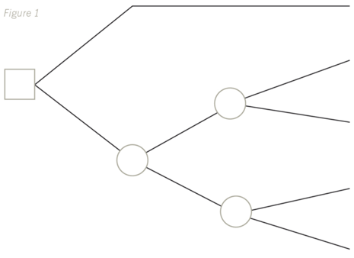
Once the basic tree has been drawn, like above, the probabilities and expected values must be written on it. Remember, the probabilities shown on the branches coming off the outcome points must always add up to 100%, otherwise there must be an outcome missing or a mistake with the numbers being used. As well as showing the probabilities on the branches of the tree, the relevant cash inflows/outflows must also be written on there too. This is shown in the example later on in the article.
Once the decision tree has been drawn, the decision must then be evaluated.
EVALUATING THE DECISION
When a decision tree is evaluated, the evaluation starts on the right-hand side of the page and moves across to the left – ie in the opposite direction to when the tree was drawn. The steps to be followed are as follows:
- Label all of the decision and outcome points – ie all the squares and circles. Start with the ones closest to the right-hand side of the page, labelling the top and then the bottom ones, and then move left again to the next closest ones.
- Then, moving from right to left across the page, at each outcome point, calculate the expected value of the cashflows by applying the probabilities to the cashflows. If there is room, write these expected values on the tree next to the relevant outcome point, although be sure to show all of your workings for them clearly beneath the tree too.
Finally, the recommendation is made to management, based on the option that gives the highest expected value.
It is worth remembering that using expected values as the basis for making decisions is not without its limitations. Expected values give us a long run average of the outcome that would be expected if a decision was to be repeated many times. So, if we are in fact making a one-off decision, the actual outcome may not be very close to the expected value calculated and the technique is therefore not very accurate. Also, estimating accurate probabilities is difficult because the exact situation that is being considered may not well have arisen before.
The expected value criterion for decision making is useful where the attitude of the investor is risk neutral. They are neither a risk seeker nor a risk avoider. If the decision maker’s attitude to risk is not known, it difficult to say whether the expected value criterion is a good one to use. It may in fact be more useful to see what the worst-case scenario and best-case scenario results would be too, in order to assist decision making.
Let me now take you through a simple decision tree example. For the purposes of simplicity, you should assume that all of the figures given are stated in net present value terms.
Example
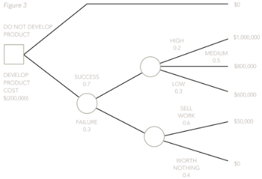
A company is deciding whether to develop and launch a new product. Research and development costs are expected to be $400,000 and there is a 70% chance that the product launch will be successful, and a 30% chance that it will fail. If it is successful, the levels of expected profits and the probability of each occurring have been estimated as follows, depending on whether the product’s popularity is high, medium or low:
| Probability | Profits | |
|---|---|---|
| High: | 0.2 | $500,000 per annum for two years |
| Medium: | 0.5 | $400,000 per annum for two years |
| Low: | 0.3 | $300,000 per annum for two years |
If it is a failure, there is a 0.6 probability that the research and development work can be sold for $50,000 and a 0.4 probability that it will be worth nothing at all.
The basic structure of the decision tree must be drawn, as shown below:
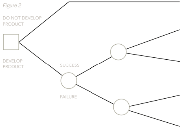
Next, the probabilities and the profit figures must be put on, not forgetting that the profits from a successful launch last for two years, so they must be doubled.
Now, the decision points and outcome points must be labelled, starting from the right-hand side and moving across the page to the left.
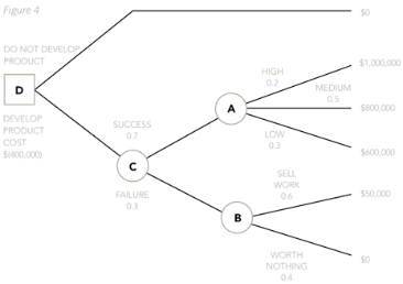
Now, calculate the expected values at each of the outcome points, by applying the probabilities to the profit figures. An expected value will be calculated for outcome point A and another one will be calculated for outcome point B. Once these have been calculated, a third expected value will need to be calculated at outcome point C. This will be done by applying the probabilities for the two branches off C to the two expected values that have already been calculated for A and B.
EV at A = (0.2 x $1,000,000) + (0.5 x $800,000) + (0.3 x $600,000) = $780,000.
EV at B = (0.6 x $50,000) + (0.4 x $0) = $30,000.
EV at C = (0.7 x $780,000) + (0.3 x $30,000) = $555,000
These expected values can then be put on the tree if there is enough room.
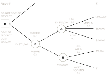
Once this has been done, the decision maker can then move left again to decision point D. At D, the decision maker compares the value of the top branch of the decision tree (which, given there were no outcome points, had a certain outcome and therefore needs no probabilities to be applied to it) to the expected value of the bottom branch. Costs will then need to be deducted. So, at decision point D compare the EV of not developing the product, which is $0, with the EV of developing the product once the costs of $400,000 have been taken off – ie $155,000.
Finally, the recommendation can be made to management. Develop the product because the expected value of the profits is $155,000.
Often, there is more than one way that a decision tree could be drawn. In my example, there are actually five outcomes if the product is developed:
- It will succeed and generate high profits of $1,000,000.
- It will succeed and generate medium profits of $800,000.
- It will succeed and generate low profits of $600,000.
- It will fail but the work will be sold generating a profit of $50,000.
- It will fail and generate no profits at all.
Therefore, instead of decision point C having only two branches on it, and each of those branches in turn having a further outcome point with two branches on, we could have drawn the tree as follows:
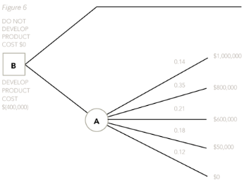
You can see that the probabilities on the branches of the tree coming off outcome point A are now new. This is because they are joint probabilities and they have been by combining the probabilities of success and failure (0.7 and 0.3) with the probabilities of high, medium and low profits (0.2, 0.5, 0.3). The joint probabilities are found easily simply by multiplying the two variables together each time:
Success and high profits: 0.7 x 0.2 = 0.14
Success and medium profits: 0.7 x 0.5 = 0.35
Success and low profits: 0.7 x 0.3 = 0.21
Fail and sell works: 0.3 x 0.6 = 0.18
Fail and don’t sell work: 0.3 x 0.4 = 0.12
All of the joint probabilities above must, of course, add up to 1, otherwise a mistake has been made.
Whether you use my initial method, which I always think is far easier to follow, or the second method, your outcome will always be the same.
The decision tree example above is quite a simple one but the principles to be grasped from it apply equally to a more complex decision resulting in a tree with far more decision points, outcomes and branches on.
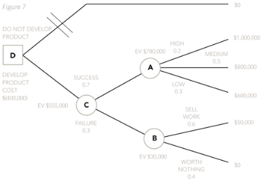
Finally, I always cross off the branch or branches after a decision point that show the alternative I haven’t chosen, in this case being the ‘do not develop product’ branch. Not everyone does it this way but I think it makes the tree easy to follow. Remember, outcomes are not within your control, so branches off outcome points are never crossed off. I have shown this crossing off of the branches below on my original, preferred tree:
THE VALUE OF PERFECT AND IMPERFECT INFORMATION
Perfect information is said to be available when a 100% accurate prediction can be made about the future. Imperfect information, on the other hand, is not 100% accurate but provides more knowledge than no information. Imperfect information is far more difficult to calculate and you would only ever need to do this in the exam if the numbers were extremely straightforward to start with. In this article, we are only going to deal with perfect information in any detail. This is because the calculations involved in calculating the value of imperfect information from my example are more complex than the Paper F5 syllabus would require you to calculate.
Perfect information
The value of perfect information is the difference between the expected value of profit with perfect information and the expected value of profit without perfect information. So, in our example, let us say that an agency can provide information on whether the launch is going to be successful and produce high, medium or low profits or whether it is simply going to fail. The expected value with perfect information can be calculated using a small table. At this point, it is useful to have calculated the joint probabilities mentioned in the second decision tree method above because the answer can then be shown like this.
| Success of failure and demand level | Joint probability | Profit less cost | Proceed | EV of info |
|---|---|---|---|---|
| Success and high | 0.14 | $600,000 | Yes | $84,000 |
| Success and medium | 0.35 | $400,000 | Yes | $140,000 |
| Success and low | 0.21 | $200,000 | Yes | $42,000 |
| Fail and sell | 0.18 | $(350,000) | No | 0 |
| Fail and don't sell | 0.12 | $(400,000) | No | 0 |
| $266,000 |
However, it could also be done by using the probabilities from our original tree in the table below and then multiplying them by the success and failure probabilities of 0.7 and 0.3:
| Demand level | Probability | Profit less development cost | Proceed | EV of info |
|---|---|---|---|---|
| High | 0.2 | $600,000 | Yes | $120,000 |
| Medium | 0.5 | $400,000 | Yes | $200,000 |
| Low | 0.3 | $200,000 | Yes | $60,000 |
| $380,000 |
EV of success with perfect information = 0.7 x $380,000 = $266,000
| Demand level | Probability | Profit less development cost | Proceed | EV of info |
|---|---|---|---|---|
| Fail and sell | 0.6 | $(350,000) | No | 0 |
| Fail and don't sell | 0.4 | $(400,000) | No | 0 |
| Expected value | $0 |
EV of failure with perfect information = 0.3 x $0 = $0.
Therefore, total expected value with perfect information = $266,000.
Whichever method is used, the value of the information can then be calculated by deducting the expected value of the decision without perfect information from the expected value of the decision with perfect information – ie $266,000 – $155,000 = $111,000. This would represent the absolute maximum that should be paid to obtain such information.
Imperfect information
In reality, information obtained is rarely perfect and is merely likely to give us more information about the likelihood of different outcomes rather than perfect information about them. However, the numbers involved in calculating the values of imperfect information are rather complex and at Paper F5 level, any numerical question would need to be relatively simple. You should refer to the recommended text for a worked example on the value of imperfect information. It is suffice here to say that the value of imperfect information will always be less than the value of perfect information unless both are zero. This would occur when the additional information would not change the decision. Note that the principles that are applied for calculating the value of imperfect information are the same as those applied for calculating the value of perfect information.





 白金级认可培训资质(总部)
 课程试听
课程试听
 职业规划
职业规划
 ACCA中文教材
 考位预约
考位预约
 免费资料
免费资料


 题库下载
题库下载
 模拟机考
模拟机考


 CFA®成绩查询


 GARP协会官方认可FRM®备考机构


